| Type: | Package |
| Title: | Efficient Algorithm for High-Dimensional Frailty Model |
| Version: | 1.2.1 |
| Maintainer: | Yunpeng Zhou <u3514104@connect.hku.hk> |
| Description: | The penalized and non-penalized Minorize-Maximization (MM) method for frailty models to fit the clustered data, multi-event data and recurrent data. Least absolute shrinkage and selection operator (LASSO), minimax concave penalty (MCP) and smoothly clipped absolute deviation (SCAD) penalized functions are implemented. All the methods are computationally efficient. These general methods are proposed based on the following papers, Huang, Xu and Zhou (2022) <doi:10.3390/math10040538>, Huang, Xu and Zhou (2023) <doi:10.1177/09622802221133554>. |
| License: | GPL-2 | GPL-3 [expanded from: GPL (≥ 2)] |
| Encoding: | UTF-8 |
| LazyData: | false |
| Depends: | R (≥ 3.5.0), survival, numDeriv, mgcv |
| Imports: | Rcpp (≥ 1.0.8), utils, graphics, stats |
| LinkingTo: | Rcpp, RcppGSL |
| RoxygenNote: | 7.2.3 |
| NeedsCompilation: | yes |
| Packaged: | 2023-08-08 07:51:11 UTC; micha |
| Author: | Xifen Huang [aut], Yunpeng Zhou [aut, cre], Jinfeng Xu [ctb] |
| Repository: | CRAN |
| Date/Publication: | 2023-08-08 09:10:02 UTC |
cluster function
Description
Specify cluster id for clustered data or object id for recurrent data in the input formula.
Usage
cluster(x)
Arguments
x |
name from original dataframe which specifies the cluster or object id. |
Value
No return value, called to construct formula.
retrieve the coefficients under given tuning parameter
Description
retrieve the coefficients under given tuning parameter
Usage
## S3 method for class 'fpen'
coef(object, ...)
Arguments
object |
Object with class "fpen", generated from |
... |
Ignored |
Details
Without given a specific tune value, the coefficients with minimum BIC is returned. If tune=a,
the coefficient is computed using linear interpolation of the result from the coefficients estimated from the run of regularization path.
Thus, a should between the minimum and maximum value of the tuning parameter sequences used for the model fitting.
Value
A vector of estimated parameters.
event function
Description
Specify event id for multi-event data in the input formula.
Usage
event(x)
Arguments
x |
name from original dataframe which specifies the event id. |
Value
No return value, called to construct formula.
Fitting frailty models with clustered, multi-event and recurrent data using MM algorithm
Description
This formula is used to fit the non-penalized regression. 3 types of the models can be fitted, shared frailty model where
hazard rate of j^{th} object in i^{th} cluster is
\lambda_{ij}(t|\omega_i) = \lambda_0(t) \omega_i \exp(\boldsymbol{\beta}' \mathbf{X_{ij}}).
The multi-event frailty model with different baseline hazard of different event and the hazard rate of j^{th} event for individual i^{th} is
\lambda_{ij}(t|\omega_i) = \lambda_{0j}(t) \omega_i \exp(\boldsymbol{\beta}' \mathbf{X_{ij}}).
The recurrent event model where the j^{th} event of individual i has observed feature \mathbf{X_{ij}},
\lambda_{ij}(t|\omega_i) = \lambda_0(t) \omega_i \exp(\boldsymbol{\beta}' \mathbf{X_{ij}}).
For the clustered type of data, we further assume that cluster i has n_i with j=1,...,n_{i} number
of objects where they share the common frailty parameter \omega_i. For simplicity, we let \boldsymbol{\alpha}
be the collection of all parameters and baseline hazard function. Then, the marginal likelihood is as follows,

Given the objective functions above, we take the clustered data as an example to illustrate the application of MM algorithm in optimizing the observed likelihood function, the observed log-likelihood function is,

where,

In order to formulate the iterative algorithm to optimize the observed log likelihood, we further define density function g_i(\cdot)
based on the estimates of the parameters in k^{th} iteration \boldsymbol{\alpha}^{(k)}

Then, we construct the surrogate function to minimize the mariginal log-likelihood using the Jensen's inequality,
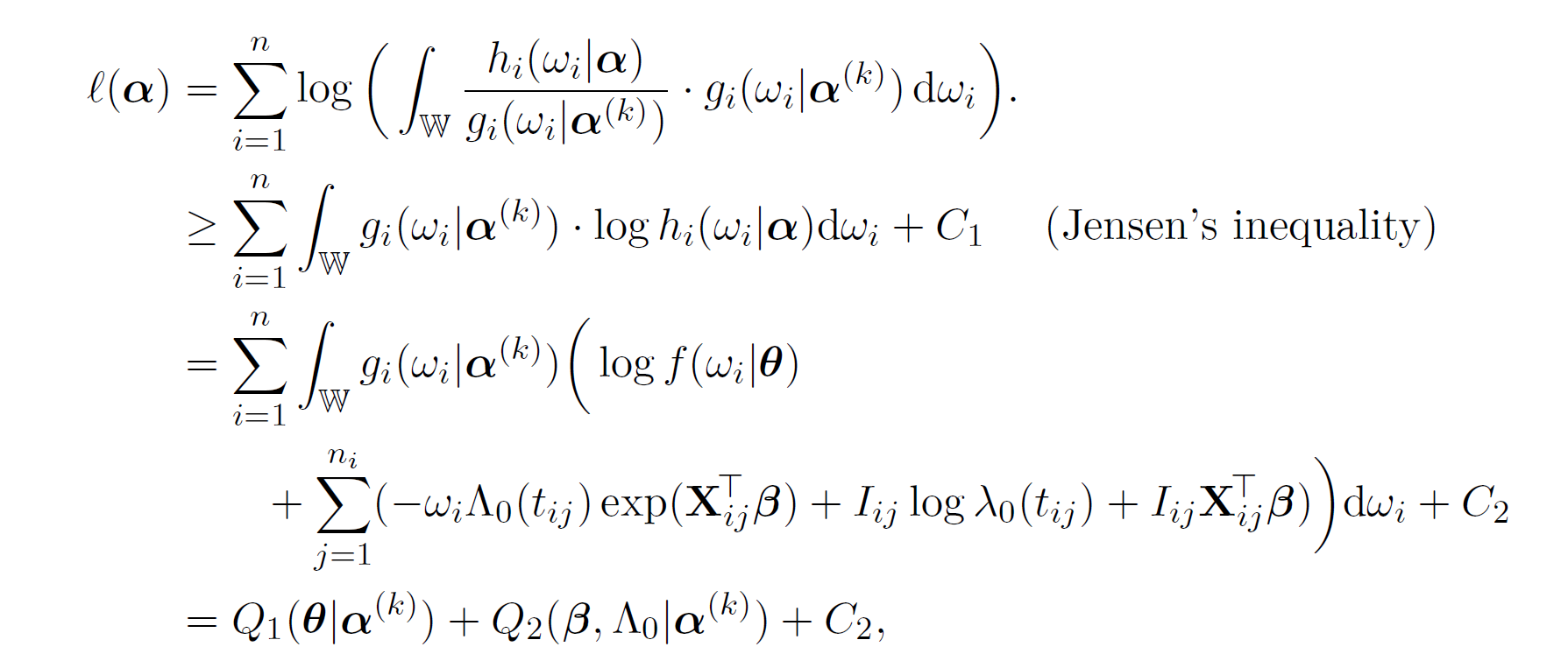
which successfully separated \boldsymbol{\alpha} into \boldsymbol{\theta} and (\boldsymbol{\beta}, \Lambda_{0}) where,

and let 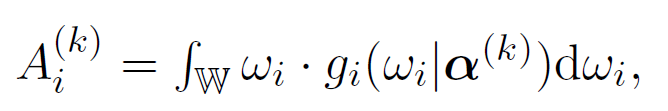 ,
,

And then we estimate \Lambda_{0} by,

Then, we have,

Further more, we apply hyperplane inequality to construct surrogate function for \boldsymbol{\beta} where we can update the its estimates coordinate wise,

By applying Jensen's inequality,

Finally,

Usage
frailtyMM(
  formula,
  data,
  frailty = "gamma",
  power = NULL,
  tol = 1e-05,
  maxit = 200,
  ...
)
Arguments
formula |
Formula where the left hand side is an object of the type |
data |
The |
frailty |
The frailty used for model fitting. The default is "lognormal", other choices are "invgauss", "gamma" and "pvf". (Note that the computation time for PVF family will be slow due to the non-explicit expression of likelihood function) |
power |
The power used if PVF frailty is applied. |
tol |
The tolerance level for convergence. |
maxit |
Maximum iterations for MM algorithm. |
... |
additional arguments pass to the function. |
Details
To run the shared frailty model, Surv(tstop, status) formula should be applied along with +cluster() to specify the
corresponding clusters, if you want to run the simple frailty model without shared frailty, you do not need to use +cluster() and the
formula only contains the name of the covariates. To run the multi-event model,
Surv(tstop, status) formula should be applied along with +event() to specify the corresponding events. If multi-event data
is fitted, please use 1,2...,K to denote the event id from the input data. To run the recurrent event model,
Surv(tstart, tstop, status) formula should be applied along with +cluster() where the cluster here denotes the individual id and
each individual may have many observed events at different time points.
The default frailty will be log-normal frailty, in order to fit other frailty models, simply set parameter frailty as "InvGauss", "Gamma" or "PVF",
the parameter power is only used when frailty=PVF and since the likelihood of PVF (tweedie) distribution is approximated using
Tweedie function from package mgcv, 1<power<2.
Value
An object of class fmm that contains the following fields:
coef |
coefficient estimated from a specific model. |
est.tht |
frailty parameter estimated from a specific model. |
lambda |
frailty for each observation estimated from a specific model. |
likelihood |
The observed log-likelihood given estimated parameters. |
input |
The input data re-ordered by cluster id. |
frailty |
frailty used for model fitting. |
power |
power used for model fitting is PVF frailty is applied. |
iter |
total number of iterations. |
convergence |
convergence threshold. |
formula |
formula applied as input. |
coefname |
name of each coefficient from input. |
id |
id for individuals or clusters, 1,2...,a. Note that, since the original id may not be the sequence starting from 1, this output
id may not be identical to the original id. Also, the order of id is corresponding to the returned |
N |
total number of observations. |
a |
total number of individuals or clusters. |
datatype |
model used for fitting. |
References
Huang, X., Xu, J. and Zhou, Y. (2022). Profile and Non-Profile MM Modeling of Cluster Failure Time and Analysis of ADNI Data. Mathematics, 10(4), 538.
Huang, X., Xu, J. and Zhou, Y. (2023). Efficient algorithms for survival data with multiple outcomes using the frailty model. Statistical Methods in Medical Research, 32(1), 118-132.
Examples
# Kidney data fitted by Clustered Inverse Gaussian Frailty Model


InvG_real_cl = frailtyMM(Surv(time, status) ~ age + sex + cluster(id),
                         kidney, frailty = "invgauss")
InvG_real_cl

# Cgd data fitted by Recurrent Log-Normal Frailty Model

logN_real_re = frailtyMM(Surv(tstart, tstop, status) ~ sex + treat + cluster(id),
                         cgd, frailty = "gamma")
logN_real_re


# Simulated data example

data(simdataCL)

# Parameter estimation under different model structure and frailties

# Clustered Gamma Frailty Model
gam_cl = frailtyMM(Surv(time, status) ~ . + cluster(id),
                   simdataCL, frailty = "gamma")


# Clustered Log-Normal Frailty Model
logn_cl = frailtyMM(Surv(time, status) ~ . + cluster(id),
                    simdataCL, frailty = "lognormal")

# Clustered Inverse Gaussian Frailty Model
invg_cl = frailtyMM(Surv(time, status) ~ . + cluster(id),
                    simdataCL, frailty = "invgauss")

data(simdataME)

# Multi-event Gamma Frailty Model
gam_me = frailtyMM(Surv(time, status) ~ . + cluster(id),
                   simdataCL, frailty = "gamma")


# Multi-event Log-Normal Frailty Model
logn_me = frailtyMM(Surv(time, status) ~ . + event(id),
                    simdataME, frailty = "lognormal")

# Multi-event Inverse Gaussian Frailty Model
invg_me = frailtyMM(Surv(time, status) ~ . + event(id),
                    simdataME, frailty = "invgauss")

data(simdataRE)

# Recurrent event Gamma Frailty Model
gam_re = frailtyMM(Surv(start, end, status) ~ . + cluster(id),
                   simdataRE, frailty = "gamma")

# Recurrent event Log-Normal Frailty Model
logn_re = frailtyMM(Surv(start, end, status) ~ . + cluster(id),
                   simdataRE, frailty = "lognormal")

# Recurrent event Inverse Gaussian Frailty Model
invg_re = frailtyMM(Surv(start, end, status) ~ . + cluster(id),
                    simdataRE, frailty = "invgauss")


# Obtain the summary statistics under fitted model

coef(gam_cl)
summary(gam_cl)
Fitting penalized frailty models with clustered, multi-event and recurrent data using MM algorithm
Description
This formula is used to fit the penalized regression. 3 types of the models can be fitted similar to the function
frailtyMM. In addition, variable selection can be done by three types of penalty, LASSO, MCP and SCAD with the following
objective function where \lambda is the tuning parameter and q is the dimension of \boldsymbol{\beta},
l(\boldsymbol{\beta},\Lambda_0|Y_{obs}) - n\sum_{p=1}^{q} p(|\beta_p|, \lambda).
The BIC is computed using the following equation,
-2l(\hat{\boldsymbol{\beta}}, \hat{\Lambda}_0) + G_n(\hat{S}+1)\log(n),
where G_n=\max\{1, \log(\log(q+1))\} and \hat{S} is the degree of freedom.
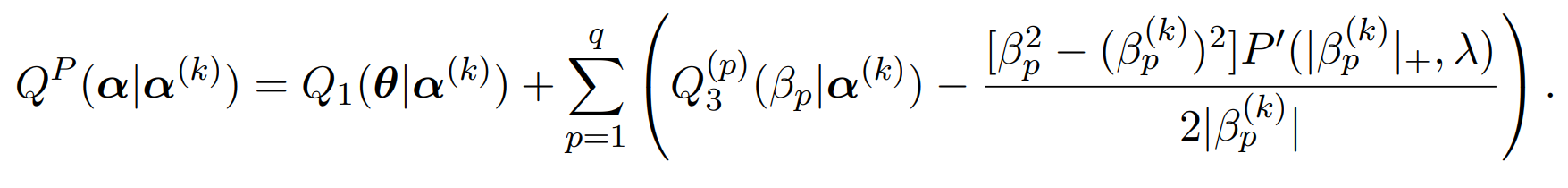
Surrogate function is also derived for penalty part for efficient estimation of penalized regression, similar to the notation used
in frailtyMM, we let \boldsymbol{\alpha} be the collection of all parameters and baseline hazard function. Given that,

by local quadratic approximation,

And thus, the surrogate function given k^{th} iteration result is as follows,
Usage
frailtyMMpen(
  formula,
  data,
  frailty = "gamma",
  power = NULL,
  penalty = "LASSO",
  gam = NULL,
  tune = NULL,
  tol = 1e-05,
  maxit = 200,
  ...
)
Arguments
formula |
Formula where the left hand side is an object of the type |
data |
The |
frailty |
The frailty used for model fitting. The default is "lognormal", other choices are "invgauss", "gamma" and "pvf". (Note that the computation time for PVF family will be slow due to the non-explicit expression of likelihood function) |
power |
The power used if PVF frailty is applied. |
penalty |
The penalty used for regularization, the default is "LASSO", other choices are "MCP" and "SCAD". |
gam |
The tuning parameter for MCP and SCAD which controls the concavity of the penalty. For MCP,
and for "SCAD",
The default value of |
tune |
The sequence of tuning parameters provided by user. If not provided, the default grid will be applied. |
tol |
The tolerance level for convergence. |
maxit |
Maximum iterations for MM algorithm. |
... |
additional arguments pass to the function. |
Details
Without a given tune, the default sequence of tuning parameters are used to provide the regularization path.
The formula is same as the input for function frailtyMM.
Value
An object of class fmm that contains the following fields:
coef |
matrix of coefficient estimated from a specific model where each column correponds to an input tuning parameter. |
est.tht |
vector of frailty parameters estimated from a specific model with respect to each tuning parameter. |
lambda |
list of frailty for each observation estimated from a specific model with respect to each tuning parameter. |
likelihood |
vector of the observed log-likelihood given estimated parameters with respect to each tuning parameter. |
BIC |
vector of the BIC given estimated parameters with respect to each tuning parameter. |
tune |
vector of tuning parameters used for penalized regression. |
tune.min |
tuning parameter where minimal of BIC is obtained. |
convergence |
convergence threshold. |
input |
The input data re-ordered by cluster id. |
y |
input stopping time. |
X |
input covariate matrix. |
d |
input censoring indicator. |
formula |
formula applied as input. |
coefname |
name of each coefficient from input. |
id |
id for individuals or clusters, 1,2...,a. Note that, since the original id may not be the sequence starting from 1, this output
id may not be identical to the original id. Also, the order of id is corresponding to the returned |
N |
total number of observations. |
a |
total number of individuals or clusters. |
datatype |
model used for fitting. |
References
Huang, X., Xu, J. and Zhou, Y. (2022). Profile and Non-Profile MM Modeling of Cluster Failure Time and Analysis of ADNI Data. Mathematics, 10(4), 538.
Huang, X., Xu, J. and Zhou, Y. (2023). Efficient algorithms for survival data with multiple outcomes using the frailty model. Statistical Methods in Medical Research, 32(1), 118-132.
See Also
Examples
data(simdataCL)

# Penalized regression under clustered frailty model

# Clustered Gamma Frailty Model

# Using default tuning parameter sequence
gam_cl1 = frailtyMMpen(Surv(time, status) ~ . + cluster(id),
                       simdataCL, frailty = "gamma")


# Using given tuning parameter sequence
gam_cl2 = frailtyMMpen(Surv(time, status) ~ . + cluster(id),
                       simdataCL, frailty = "gamma", tune = 0.1)

# Obtain the coefficient where minimum BIC is obtained
coef(gam_cl1)

# Obtain the coefficient with tune = 0.2.
coef(gam_cl1, tune = 0.2)

# Plot the regularization path
plot(gam_cl1)

# Get the degree of freedom and BIC for the sequence of tuning parameters provided
print(gam_cl1)
Simulated High-dimensional Clustered data
Description
This data include 50 clusters with 4 objects, a total of 200 events are recorded. 500 covariates can be used for model fitting. The data is generated from a gamma frailty model with coefficients (5,5,5,5,...,0) and frailty variance 1.
Usage
data(hdCLdata)
Format
An object of class data.frame with 200 rows and 503 columns.
Examples
data(hdCLdata)
Plot the baseline hazard or the predicted hazard based on the new data
Description
Both the cumulative hazard and the survival curves can be plotted.
Usage
##S3 method for class "fmm"
Arguments
newdata |
The new data for prediction of hazard |
surv |
Plot survival curve instead of cumulative hazard, the default is |
... |
Further arguments pass to or from other methods |
object |
Object with class "fmm" |
Details
If parameter newdata is given, the plot is based on the predicted hazard while if it is not given,
the plot is based on the baseline hazard. To construct the new data, please refer to the detailed description from
function predict.fmm and the following example.
See Also
Examples
gam_re = frailtyMM(Surv(tstart, tstop, status) ~  sex + treat + cluster(id), cgd, frailty = "gamma")

# Plot the survival curve based on baseline hazard
plot(gam_re, surv = TRUE)

# Construct new data and plot the cumulative hazard based on new data
newre = c(1, 1, 2)
names(newre) = c(gam_re$coefname, "id")
plot(gam_re, newdata = newre)
Plot the regularization path
Description
Plot the whole regularization path run by frailtyMMpen
Usage
##S3 method for class "fpen"
Arguments
x |
Object with class "fpen" |
... |
Further arguments pass to or from other methods |
Estimate the baseline hazard or the predict hazard rate based on the new data for non-penalized regression
Description
This function is used to estimate the baseline hazard or to predict the hazard rate of a specific individual given result from model fitting.
Usage
##S3 method for class "fmm"
Arguments
object |
Object with class "fmm" |
newdata |
The new data for prediction of hazard, categorical data has to be transformed to 0 and 1 |
surv |
Plot survival curve instead of cumulative hazard, the default is |
... |
Further arguments pass to or from other methods |
Details
If parameter newdata is given, the predicted hazard is calculated based on the given data.
If parameter newdata is not given, the estimation of baseline hazard will be returned.
The confidence band is calculated based on the delta method. Please insure that the input of new data
should be of the same coefficient name as object$coefname. Note that if original data contains categorical data, you could check
object$coefname to input the corresponding 0 or 1 and name of coefficient for the newdata.
For example, if the coefficient name is "sexfemale", then 1 denotes female while 0 denotes male. You may refer to the
example below to construct the new data.
Value
output |
A dataframe that the first column is the evaluated time point, the second column is the estimated cumulative hazard or survival curve, the third column is the standard error of the estimation result and the fourth and fifth column are the lower bound and upper bound based on 95 percent confidence interval. |
Examples
gam_re = frailtyMM(Surv(tstart, tstop, status) ~  sex + treat + cluster(id), cgd, frailty = "Gamma")

# Calculate the survival curve based on baseline hazard
predict(gam_re, surv = TRUE)

# Construct new data and calculate the cumulative hazard based on new data
newre = c(1, 1, 2)
names(newre) = c(gam_re$coefname, "id")
predict(gam_re, newdata = newre)
Estimate the baseline hazard or the predict hazard rate based on the new data for penalized regression
Description
This function is used to estimate the baseline hazard or to predict the hazard rate of a specific individual given result from model fitting.
Usage
##S3 method for class "fpen"
Arguments
object |
Object with class "fpen" |
tune |
The tuning parameter for estimating coefficients |
coef |
Instead of providing tuning parameter, you can directly provide the coefficients for prediction |
newdata |
The new data for prediction of hazard, categorical data has to be transformed to 0 and 1 |
surv |
Plot survival curve instead of cumulative hazard, the default is |
... |
Further arguments pass to or from other methods |
Details
If parameter newdata is given, the predicted hazard is calculated based on the given data.
If parameter newdata is not given, the estimation of baseline hazard will be returned.
Since the covariance of estimated parameters for penalized regression cannot be obtained from MLE theorem, we
only provide the estimation without confidence band. For the formulation of new data, you may refer to
function predict.fmm for detailed description.
Value
output |
A dataframe that the first column is the evaluated time point and the second column is the estimated cumulative hazard or survival curve. |
Examples
data(simdataCL)


gam_cl = frailtyMMpen(Surv(time, status) ~  . + cluster(id), simdataCL, frailty = "Gamma")

# Calculate the survival curve based on baseline hazard
predict(gam_cl, surv = TRUE)

# Construct new data and calculate the cumulative hazard based on new data
newcl = c(gam_cl$X[1,], 2)
names(newcl) = c(gam_cl$coefname, "id")
predict(gam_cl, newdata = newcl)
print a non-penalized regression object
Description
Print the summary of a non-penalized regression fitted by any model with function frailtyMM
Usage
## S3 method for class 'fmm'
print(x, ...)
Arguments
x |
Object with class "fmm" fitted by function |
... |
Ignored |
Value
No return value, called to print the summary for non-penalized regression.
See Also
print a penalized regression object
Description
Print the summary of a non-penalized regression fitted by any model with function frailtyMMpen.
The first column is the tuning parameter sequence, the second column is the degree of freedom and the third column is the BIC.
Usage
## S3 method for class 'fpen'
print(x, ...)
Arguments
x |
Object with class "fpen" fitted by function |
... |
Ignored |
Value
No return value, called to print the summary for penalized regression.
See Also
Simulated Clustered data
Description
This data include 50 clusters with 10 objects, a total of 100 events are recorded. 30 temporal covariates can be used for model fitting. The data is generated from a gamma frailty model with coefficients (1,2,3,4,0,...,0) and frailty variance 1.
Usage
data(simdataCL)
Format
An object of class data.frame with 500 rows and 33 columns.
Examples
data(simdataCL)
Simulated Multiple Event data
Description
This data include 50 individuals with 2 events, a total of 100 events are recorded. 30 temporal covariates can be used for model fitting. The data is generated from a gamma frailty model with coefficients (1,2,3,4,0,...,0) and frailty variance 1.
Usage
data(simdataME)
Format
An object of class data.frame with 100 rows and 33 columns.
Examples
data(simdataME)
Simulated Recurrent Event data
Description
This data include 50 individuals with recurrent observation of events, a total of 706 events are recorded. 30 temporal covariates can be used for model fitting. The data is generated from a gamma frailty model with coefficients (1,2,3,4,0,...,0) and frailty variance 1.
Usage
data(simdataRE)
Format
An object of class data.frame with 706 rows and 34 columns.
Examples
data(simdataRE)
Provide the summary for the model fitting
Description
Provide the summary for the model fitting
Usage
##S3 method for class "fmm"
Arguments
object |
Object with class "fmm", generated from |
... |
Ignored |
Details
the summary for the model of frailtyMM. The standard error and p-value of estimated parameters are based on Fisher Information matrix.