Bratteli graphs.
![]()
This package deals with Bratteli
graphs. In every function of the package, the Bratteli graph is
given by a function returning for a level n of the graph
the incidence matrix of the graph between level n and level
n+1: the (i,j)-entry of this matrix is the
number of edges between the i-th vertex at level
n and the j-th vertex at level
n+1.
For example, the binary tree is defined by:
tree <- function(n) {
  M <- matrix(0, nrow = 2^n, ncol = 2^(n+1))
  for(i in 1:nrow(M)) {
    M[i, ][c( 2*(i-1)+1, 2*(i-1)+2 )] <- 1
  }
  M
}
The function bratteliGraph generates some LaTeX code
which renders the graph up to a given level:
bratteliGraph("binaryTree.tex", tree, 3)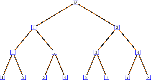
If you don’t like the style, you are free to modify the LaTeX code.
Here is a binary tree with double edges:
tree2 <- function(n) {
  M <- matrix(0, nrow = 2^n, ncol = 2^(n+1))
  for(i in 1:nrow(M)) {
    M[i, ][c( 2*(i-1)+1, 2*(i-1)+2 )] <- 2
  }
  M
}
bratteliGraph("binaryTree2.tex", tree2, 3)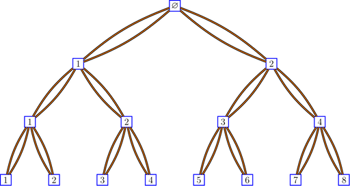
Here is the code for the Pascal graph:
Pascal <- function(n) {
  M <- matrix(0, nrow = n+1, ncol = n+2)
  for(i in 1:(n+1)) {
    M[i, ][c( i, i+1L )] <- 1
  }
  M
}
The dimension of a vertex of a Bratteli graph is the number
of paths of the graph going from the root vertex to this vertex. The
function bratteliDimensions of the package computes these
numbers:
library(bratteli)
bratteliDimensions(Pascal, 3)
## [[1]]
## [1] "1" "1"
##
## [[2]]
## [1] "1" "2" "1"
##
## [[3]]
## [1] "1" "3" "3" "1"Bratteli graphs are of interest to ergodicians, and particularly to Vershik, who introduced the intrinsic kernels of a Bratteli graph and the intrinsic distance between the vertices of a Bratteli graph. Here is a picture of the Pascal graph showing the intrinsic kernels:
bratteliGraph("Pascal.tex", Pascal, 3, edgelabels = "kernels")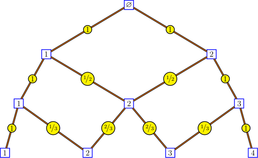
The intrinsic kernels are returned by the function
bratteliKernels. The intrinsic distances between two
vertices at the same level are returned by the function
bratteliDistances.