| Type: | Package |
| Title: | R Cross Entropy Inspired Method for Optimization |
| Version: | 0.3 |
| Date: | 2017-04-03 |
| Author: | Alberto Krone-Martins |
| Maintainer: | Alberto Krone-Martins <algol@sim.ul.pt> |
| Description: | An implementation of a stochastic heuristic method for performing multidimensional function optimization. The method is inspired in the Cross-Entropy Method. It does not relies on derivatives, neither imposes particularly strong requirements into the function to be optimized. Additionally, it takes profit from multi-core processing to enable optimization of time-consuming functions. |
| License: | GPL-2 | GPL-3 [expanded from: GPL (≥ 2)] |
| Suggests: | parallel |
| NeedsCompilation: | no |
| Packaged: | 2017-04-03 19:00:59 UTC; algol |
| Repository: | CRAN |
| Date/Publication: | 2017-04-03 20:19:16 UTC |
An R Cross Entropy Inspired Method for Optimization RCEIM
Description
RCEIM is a package implementing a stochastic heuristic method for performing multidimensional function optimization. The method is inspired in the Cross-Entropy Method.
Details
| Package: | RCEIM |
| Type: | Package |
| Version: | 0.3 |
| Date: | 2015-02-19 |
| License: | GPL (>= 2) |
RCEIM implements a simple stochastic heuristic method for optimization in the function ceimOpt. This method starts from a random population of solutions, computes the values of the function and selects a fraction of these solutions - the elite members. Afterwards, based on the elite members it creates a gaussian distribution, samples new random solutions from it, and iterates until convergence is reached (this is controlled by an epsilon parameter) or other stopping criteria is fulfilled (such as the maximum number of iterations).
One advantage of this method is that it does not impose strong conditions on the function to be optimized. The function must written as an R function, but it does not need to be continuous, differentiable, neither analytic. Moreover, the method is ready for multicore processing, enabling the optimization of time-consuming functions.
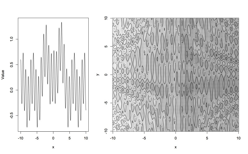
Two examples of 1D and 2D functions that can be used as test problems for RCEIM (defined in testFunOptimization and testFunOptimization2d) are represented in the above figures.
Author(s)
Alberto Krone-Martins, Laurent Gallucio
Maintainer: Alberto Krone-Martins <algol@sim.ul.pt>
See Also
Examples
# Solve a simple optimization problem and shows the results
po <- ceimOpt(OptimFunction=function(x){(x[1]+1)^2+(x[2]+2)^2}, maxIter=100, epsilon=0.3,
      nParams=2)
plotEliteDistrib(po$EliteMembers)
rm(po)

# A harder problem in 1D
po <- ceimOpt(OptimFunction="testFunOptimization", maxIter=10, epsilon=0.3,
      nParams=1, verbose=TRUE)
dev.new()
xx <- seq(-10,10,by=0.01)
plot(xx, testFunOptimization(xx), type="l", xlab="x", ylab="Value")
points(po$BestMember[1], po$BestMember[2], col="red")
rm(list=c('xx','po'))

# A harder problem in 2D
po <- ceimOpt(OptimFunction="testFunOptimization2d", maxIter=20, epsilon=0.3,
      nParams=2, verbose=TRUE)
dev.new()
xx <- seq(-10,10,by=0.1)
yy <- seq(-10,10,by=0.1)
zz <- matrix(nrow=length(yy), ncol=length(xx))
for(i in 1:length(xx)){
    for(j in 1:length(yy)){
        zz[i,j] <- testFunOptimization2d( c(xx[i],yy[j]) )
    }
}
image(xx,yy,zz, col=gray((50:100)/100), xlab="x", ylab="y")
contour(xx,yy,zz, add=TRUE)
points(po$BestMember[1], po$BestMember[2], col="red", pch=19, cex=0.5)
rm(list=c('xx','yy','zz'))

# Example of multicore processing
slowFunction <- function(x) {
  p<-runif(50000)
  return((x+3)^2)
}
system.time(po <- ceimOpt(OptimFunction="slowFunction", maxIter=10,
    Ntot=100, epsilon=0.3, nParams=1, verbose=FALSE, parallel=FALSE))
print(po$BestMember)
system.time(po <- ceimOpt(OptimFunction="slowFunction", maxIter=10,
    Ntot=100, epsilon=0.3, nParams=1, verbose=FALSE, parallel=TRUE))
print(po$BestMember)
rm(po)
A Cross Entropy Inspired Method for Optimization
Description
This is a Cross-Entropy Inspired Method for optimization.
Usage
ceimOpt(OptimFunction = "testFunOptimization", nParams = 1, minimize = TRUE,
    Ntot = 1000, N_elite = floor(Ntot/4), N_super = 1, alpha = 1, epsilon = 0.1,
    q = 2, maxIter = 50, waitGen = maxIter, boundaries = t(matrix(rep(c(-10, 10),
    nParams), ncol = nParams)),plotConvergence = FALSE, chaosGen = maxIter,
    handIterative = FALSE, verbose = FALSE, plotResultDistribution = FALSE,
    parallelVersion = FALSE)
Arguments
OptimFunction |
A string with the name of the function that will be optimized. |
nParams |
An integer with the number of parameters of the function that will be optimized. |
minimize |
A boolean indicating if the OptimFunction should be minimized or maximized. |
Ntot |
An integer with the number of individuals per iteration. |
N_elite |
An integer with the number of elite individuals, or in other words, the individuals used to define the individuals of the new iteration. |
N_super |
An integer with the number of super-individuals, or those individuals with the best fitness values, that are directly replicated to the next iteration. |
alpha |
A parameter of the CE method used to control the convergence rate, and to prevent early convergence. |
epsilon |
A convergence control parameter: if the maximum st.dev. of the parameters of the elite individuals divided by its average value is smaller than this number, the method considers that it converged. |
q |
A parameter of the CE method used to control the convergence rate, and to prevent early convergence. |
maxIter |
The maximum number of iterations that the method will run before stop. |
waitGen |
The number of iterations that the method will wait: after "waitGen" without any improvement in the best individual, the method gives up and return the best individual as an answer. |
boundaries |
A matrix with as many rows as there are parameters and two columns the first column stores the minimum value, while the second, the maximum. |
plotConvergence |
A flag to indicate if the user wants to visually check the convergence of the method. |
chaosGen |
The number of iterations before the method replaces all the solutions, but the super-individuals, by a new random trial. |
handIterative |
A flag to indicate if the user wants to press enter between the each generation. |
verbose |
A flag to indicate if the user wants to receive some convergence and distribution information printed on the screen. |
plotResultDistribution |
A flag to indicate if the user wants to see the resulting distribution of elite members (black curve), the value of the fittest member (red line) and of the average member (blue line), for each parameter. |
parallelVersion |
A flag to indicate if the user wants to use all the cores in his/her computer to compute the fitness functions. |
Details
This is a simple stochastic heuristic method for optimization. It starts from a random population of points, computes the values of the function and selects a fraction of the points - the elite members. Then, based on these fittest points, it constructs a gaussian distribution, samples new random points from it, and iterates until convergence is reached (this is controlled by the epsilon parameter) or other stopping criteria is fulfilled (such as the maximum number of iterations).
The method does not impose strong conditions on the function to be optimized. The function must written as an R function, but it does not need to be neither continuous, differentiable or analytic. Moreover, the method is ready for multicore processing, enabling the optimization of time-consuming functions.
Value
A list that contains:
BestMember |
The parameters and the fitness value of the best member. |
Convergence |
A boolean indicating if the method reached convergence. |
Criteria |
Stopping criterion. |
Iterations |
The amount of iterations. |
EliteMembers |
The parameters and fitness values of the elite members at the last iteration. |
Author(s)
Alberto Krone-Martins
Examples
# Solve a simple optimization problem and shows the results
po <- ceimOpt(OptimFunction=function(x){(x[1]+1)^2+(x[2]+2)^2}, maxIter=100, epsilon=0.3,
      nParams=2)
plotEliteDistrib(po$EliteMembers)
rm(po)

# A harder problem in 1D
po <- ceimOpt(OptimFunction="testFunOptimization", maxIter=10, epsilon=0.3,
      nParams=1, verbose=TRUE)
dev.new()
xx <- seq(-10,10,by=0.01)
plot(xx, testFunOptimization(xx), type="l", xlab="x", ylab="Value")
points(po$BestMember[1], po$BestMember[2], col="red")
rm(list=c('xx','po'))

# A harder problem in 2D
po <- ceimOpt(OptimFunction="testFunOptimization2d", maxIter=20, epsilon=0.3,
      nParams=2, verbose=TRUE)
dev.new()
xx <- seq(-10,10,by=0.1)
yy <- seq(-10,10,by=0.1)
zz <- matrix(nrow=length(yy), ncol=length(xx))
for(i in 1:length(xx)){
    for(j in 1:length(yy)){
        zz[i,j] <- testFunOptimization2d( c(xx[i],yy[j]) )
    }
}
image(xx,yy,zz, col=gray((50:100)/100), xlab="x", ylab="y")
contour(xx,yy,zz, add=TRUE)
points(po$BestMember[1], po$BestMember[2], col="red", pch=19, cex=0.5)
rm(list=c('xx','yy','zz'))

# Example of multicore processing
slowFunction <- function(x) {
  p<-runif(50000)
  return((x+3)^2)
}
system.time(po <- ceimOpt(OptimFunction="slowFunction", maxIter=10,
    Ntot=100, epsilon=0.3, nParams=1, verbose=FALSE, parallel=FALSE))
print(po$BestMember)
system.time(po <- ceimOpt(OptimFunction="slowFunction", maxIter=10,
    Ntot=100, epsilon=0.3, nParams=1, verbose=FALSE, parallel=TRUE))
print(po$BestMember)
rm(po)
Enforce domain boundaries
Description
A small function to assure that the domains are respected during the optimization process. If any of them not respected, the ofending parameters are replaced by the value of the nearest border.
Usage
enforceDomainOnParameters(paramsArray, domain)
Arguments
paramsArray |
The array with the parameters to check. |
domain |
The domain boudaries. |
Value
The parameter array, with ofending values replaced if necessary.
Author(s)
Alberto Krone-Martins
Examples
# Creates a random set of parameters in an interval larger than a certain domain
# and apply the enforceDomainOnParameters function and represent graphically
# the parameters before and after the function.
dev.new()
paramArr <- matrix((runif(100)-0.5)/0.5*13, nrow=50)
domain <- matrix(c(-10, -10, 10, 10), ncol=2)
newParamArr <- enforceDomainOnParameters(paramArr, domain)
plot(paramArr[,1], paramArr[,2], xlab="x", ylab="y", main="black: input\n red: output")
points(newParamArr[,1], newParamArr[,2], col="red", pch=19, cex=0.7)
Overplot an error polygon
Description
A simple function to overplot an error polygon around a curve. Note that the error is considered as symmetric, and exclusively on y. The polygon will be created from the coordinate tuples (x, (y - err_y)) and (x, (y + err_y)).
Usage
overPlotErrorPolygon(x, y, err_y, col = "grey", logPlot = FALSE, ...)
Arguments
x |
A vector containing the x coordinate of the data. |
y |
A vector containing the y coordinate of the data. |
err_y |
A vector containing the error in y. |
col |
The color that will be used for filling the polygon. |
logPlot |
A boolean indicating if the plot is in logscale. |
... |
Further arguments to be passed to polygon(). |
Value
A polygon is overplotted in the active graphics device.
Author(s)
Alberto Krone-Martins
Examples
# Shows a simple random curve and overplots a randomly created error bar.
dev.new()
xx <- 1:10
yy <- (1:10)/5 + 4 + (runif(10)-0.5)/0.5*2
plot(xx, yy, type="l", xlab="x", ylab="y", ylim=c(0,10))
err_yy <- 1.5 + (runif(10)-0.5)/0.5
overPlotErrorPolygon(xx,yy,err_yy, col=rgb(0,0,1,0.3), border=NA)
Plot the distribution of elite members
Description
A simple function to create distribution plots of the elite members after the optimization procedure. The distribution is graphically represented using a kernel density estimation. Aditionally, this function also indicates the best and average members.
Usage
plotEliteDistrib(elite)
Arguments
elite |
A matrix containing parameters of the elite members. |
Value
A graphic representation of the elite members and also of the best and average members.
Author(s)
Alberto Krone-Martins
See Also
Examples
# Solve a simple 2D problem and show the distribution of the parameters
po <- ceimOpt(OptimFunction=function(x){(x[1]+1)^2+(x[2]+2)^2}, maxIter=100,
      epsilon=0.1, nParams=2)
plotEliteDistrib(po$EliteMembers)
rm(po)
Sorting a data frame by a key
Description
A simple function to sort a data frame based on a certain keyword. This function was posted by r-fanatic at a dzone forum (the webpage is not available anymore).
Usage
sortDataFrame(x, key, ...)
Arguments
x |
The data frame to be sorted. |
key |
The key by which the data frame will be sorted. |
... |
Further arguments to be passed to the order function. |
Value
The sorted data frame.
Author(s)
r-fanatic
References
The original webpage where r-fanatic posted the code is not available as of 3rd April 2017.
Examples
# Create a simple data frame and order using the "B" key
ppp <- data.frame(A=1:10,B=10:1)
ppp
sortDataFrame(ppp,"B")
ppp
1D test problem for RCEIM
Description
An one-dimension problem for testing optimization methods.
This function was created for demonstrating the RCEIM package. It has the form:
f(x) = exp(-((x - 2)^2)) + 0.9 * exp(-((x + 2)^2)) + 0.5 * sin(8*x) + 0.25 * cos(2*x)
Usage
testFunOptimization(x)
Arguments
x |
The point where the function is computed. |
Value
The value of the function at x.
Author(s)
Alberto Krone-Martins
See Also
Examples
# Create a graphical representation of the problem with a line plot
dev.new()
xx <- seq(-10,10,by=0.01)
plot(xx, testFunOptimization(xx), type="l", xlab="x", ylab="Value")
rm(list=c('xx'))
2D test problem for RCEIM
Description
A two-dimensional problem for testing optimization methods.
This function was created for demonstrating the RCEIM package. It has the form:
f(x_1,x_2) = ((x_1-4)^2 + (x_2+2)^2)/50 - ((x_1+2)^2 + (x_2+4)^2)/90 -exp(-(x_1-2)^2) - 0.9*exp(-(x_2+2)^2) - 0.5*sin(8*x_1) - 0.25*cos(2*x_2) +0.25*sin(x_1*x_2/2) + 0.5*cos(x_2*x_1/2.5)
Usage
testFunOptimization2d(x)
Arguments
x |
a vector with the point where the function is computed. |
Value
The value of the function at the requested point (x_1, x_2).
Author(s)
Alberto Krone-Martins
See Also
Examples
# Create a graphical representation of the problem with a contour plot
dev.new()
xx <- seq(-10,10,by=0.1)
yy <- seq(-10,10,by=0.1)
zz <- matrix(nrow=length(yy), ncol=length(xx))
for(i in 1:length(xx)){
	for(j in 1:length(yy)){
		zz[i,j] <- testFunOptimization2d( c(xx[i],yy[j]) )
	}
}
image(xx,yy,zz, col=gray((50:100)/100), xlab="x", ylab="y")
contour(xx,yy,zz, add=TRUE)
rm(list=c('xx','yy','zz'))