03 11 2021
The original version of this software was written in R by Stanislav Zámečník, Zdeňka Geršlová and Vojtěch Šindlář in year 2021. The package is based on theoretical background of work of prof. Gejza Wimmer and afterwards implemented by mentioned authors. Main features of the package include:
You can install the release version of package from CRAN:
install.packages("OEFPIL")Or the development version from GitHub repository:
devtools::install_github("OEFPIL/OEFPIL")In R session do:
library(MASS)
steamdata <- steam
colnames(steamdata) <- c("x","y")
k <- nrow(steamdata)
CM <- diag(rep(10,2*k))
Creating OEFPIL object which we want to work with
library(OEFPIL)
st1 <- OEFPIL(steamdata, y ~ b1 * 10 ^ (b2 * x/ (b3 + x)),
list(b1 = 5, b2 = 8, b3 = 200), CM, useNLS = FALSE)
Displaying results using summary function
summary(st1)## Summary of the result:
##
## y ~ b1 * 10^(b2 * x/(b3 + x))
##
## Param Est Std Dev CI Bound 2.5 % CI Bound 97.5 %
## b1 4.487870 1.526903 1.495196 7.480545
## b2 7.188155 1.865953 3.530953 10.845356
## b3 221.837783 99.953658 25.932214 417.743352
##
## Estimated covariance matrix:
## b1 b2 b3
## b1 2.331432 2.296195 134.3054
## b2 2.296195 3.481782 184.6313
## b3 134.305405 184.631318 9990.7337
##
## Number of iterations: 10Plot of estimated function
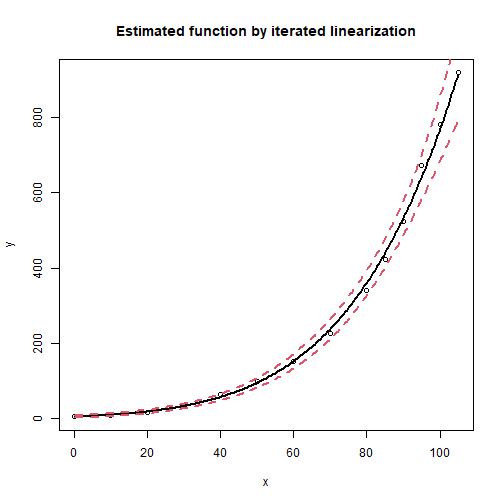
plot(st1, signif.level = 0.05, interval = "conf", main = "Estimated function by iterated linearization")
Ggplot graph of estimated function
library(ggplot2)
curvplot.OEFPIL(st1, signif.level = 0.05)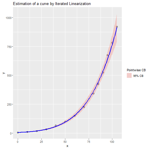
For more information and examples see:
?OEFPILThis software OEFPIL was financed by the Technology Agency of the Czech Republic within the ZETA Programme. https://www.tacr.cz .
![]()